Procedure for Phase A.2:

Details of activities:

Step A.2.1: Instrumentation [One beam at a time]

1. If not already done: move screens OUT

    

2. Commission BPM intensity measurement mode:

   • Useful to determine potential bottle-necks (in particular soft ones) and to select the data to be retained for the turn-by-turn trajectory data averaging

Step A.2.2: Establish closed orbit [One beam at a time]

1. Integer tune measurement

   • If it has not been determined from first turn data, the integer part of the tune can be measured from the difference of two orbits (one of them with a distortion from a kick) and harmonic analysis (Fourier transform) as a function of position along the ring.

    

2. Close the trajectory

   • Compare two consecutive turns (not necessarily using all BPMs for the second turn) and close the trajectory on itself with two closed orbit correctors (using YASP).

    

3. Closed orbit measurement and correction to get a few tens of turns

   • Average of the turn-by-turn data over the number of turns available (at least 10 turns).

   • Notes:

     • The BPM system can cope with an increase in r.m.s. bunch length from 0.4 to 1.3 ns, that is about 140 turns (see [1]).

     • In case of problems: reduce the Δp/p of the SPS beam in order to decrease the debunching time and thus to increase the number of turns during which beam can be seen.

    

4. Repeat for the other beam

Step A.2.3: Measurements with a few turns [One beam at a time]

1. Fractional tune measurement

   • The fractional part of the tune can be measured by exciting injection oscillations and comparing turn-by-turn trajectories or turn-by-turn phase advance measurements obtained combining the turn-by-turn data from pairs of BPMs separated by 90° in phase advance. The precision of this measurement is expected to be ΔQ=0.01 and therefore much better than the expected initial coupling (about 0.1)

    

2. Adjustment of the chromaticity

   • Correct the chromaticity at least in the horizontal plane (in order to avoid too short a de-coherence time). Any oscillation will die out rapidly because of the de-coherence due to chromaticity (the folding time grows as the square of the momentum spread):

     • <x>(n) =  exp(-0.5 α² n²) sin (2 π Q n); α = 2 π Q' σ; σ...normalized energy spread (e.g. 10^-4)

     • The e-folding time is 4 turns for natural Q'_H= -179 for σ = 3.06 10^-4. It is 43 turns for Q'_H = -17, Q'_V = 17). It can be further increased by reducing the momentum spread at extraction from SPS (88 turns for σ = 1.5 10^-4)

     • Adjust the chromaticity empirically by maximizing the de-coherence time

     • (see [1] and [2])

    

3. Adjustment of the coupling

   • Adjust the coupling empirically by exciting injection oscillations in one plane and measuring and maximizing how much is seen in the other plane: look at oscillations and try minimizing them by trial and error.

    

4. Fast physical aperture scans

   • Making use of free oscillations with BPM intensity measurement

    

5. Optional: systematic linear optics checks in case the lifetime is not sufficient

    

6. Repeat for the other beam

Step A.2.4: Offsets between different sectors [Interleaved injection]

1. Commission interleaved injection

    

2. Correction of the orbit

    

3. Correction of the Bdl sector-by-sector

   • Correct the relative octant-by-octant MB field offset down to a few 10^-4 (see [6]).

   • Note: The B-field trim should be propagated to the multipoles (at least to the quadrupoles) to keep the correct MQ-MB tracking, in order to try keeping the tune constant.

    

4. Optional: Correction of the MQ-MQ offsets sector-by-sector

   • Correct MQ-MQ offsets within LSA octant-by-octant from phase advance measurements.

   • Note: MQ-MQ tracking might be difficult to correct at this stage unless the coupling has been minimized.

Step A.2.5: RF observation equipment [One beam at a time]  (see Fig 1)

1. Keep RF OFF

    

2. Set up observation equipment and bunch reference numbers

   1. Set the observation memory to trigger on "Beam In" timing

   2. Observe the pick up signals (APW in Beam Phase module and BPM in Beam Position module).

   3. Adjust the gain/attenuation of the RF front end of the Beam Position and Beam Phase modules

   4. Align the signals from the 2 inputs

      • Easy for APW and Δ,Σ from BPM

      • More difficult for cavity sum as the beam induced voltage will be very small with pilot. Coarse adjustment must be done without beam.

   5. Adjust the F_rev marker (offset in memory addressing) so that marker points to bucket 1

Step A.2.6: SPS-LHC energy matching and Phase Loop commissioning [Mostly interleaved injection] [3x8 hours]

• Before the energy matching can start the beam must survive for at least 1/4 of a synchrotron period (that is about 45 turns at nominal voltage, that is 8MV, or about 35 turns at 16MV).

• It is assumed that one uses a common frequency for both beams in SPS and LHC (f_SPS-LHC)

• As a starting point for energy matching, the beam should be centred in the SPS at extraction and in the LHC for both rings (with RF OFF)

1. Centre the first turn in both rings

   1. RF Preparation:

      1. Keep the Synchro Loop ON

      2. Keep Phase Loop OFF

      3. Keep Radial Loop OFF

      4. Keep RF OFF

         • Note: The beam debunches in about 10 ms (100 turns)

   2. Use pilot beam with small momentum spread

   3. Centre the beam in the SPS at extraction

    

2. Measure the revolution frequency  f_rev for both beams

   • By observing the bunch slip with respect to the SPS-LHC reference frequency f_SPS-LHC / h_LHC

     • Either looking at the bunch on the longitudinal pickup:

       • Direct observation of the pickup signal.

       • The bunch phase with respect to the distributed revolution frequency is not very sensitive to the bunch length.

       • (Hardware is ready on APW platform, and pickup signal is routed to SR4)

     • Or with the phase loop discriminator versus time:

       • Using the observation memory in Beam Phase module.

       • It measures the 400 MHz component of the beam signal and will thus stop working as beam debunches (zero signal when σ_rms has increased from 0.4 ns to 0.9 ns, that is after about 100 turns. 

       • Frequency errors can be measured within about 2 Hz.

       • In case of problem, one may reduce Δp/p

   • Notes:

     • For 10^-4 dB/B ( about 0.15 mm LHC or about 15 Hz @ 400 MHz) the beam slips about 10 RF periods in 0.5 seconds.

     • The beam debunches in about 10 ms (100 turns)

     • At injection ( γ = 460,  γ_t = 53.7) a Δp/p of 10^-3 gives Δf = -120 Hz at 400 MHz and ΔR = 1.5mm

    

3. Correct Bdl_SPS, Bdl_LHC1, Bdl_LHC2, f_{RF SPSLHC}

   • Trim f_{RF SPSLHC}, the LHC integrated fields for beam 1 (Bdl_LHC1) and beam 2 (Bdl_LHC2), via the COD correctors only (see [1] and [3]), and the magnetic field at extraction in the SPS (Bdl_SPS).

   • Notes:

     • There will be a radial offset at extraction in the SPS if C_LHC differs from 27/7 C_SPS.

     • There will be a radial offset in the LHC after capture only if the two rings have a different circumference (~0.1 mm for ~1.5 mm difference).

     • 1 cm length difference corresponds to about 1.5 mm radial offset, that is to about 150 Hz

    

4. Commission the RF Phase Loop (see Fig 1)

   1. RF preparation:

      1. Switch the RF ON (with 1MV/cavity [14]).

      2. Switch the Phase Loop ON

      3. Switch the Synchro Loop OFF

   2. Observe the phase between the bunch and the total voltage V_t on the first few turns (by using the Phase Loop phase discri ΔФ_phase).

      • The phase loop will lock, but as the stable phase is wrong the beam will be accelerated or decelerated.

      • Because the RF is ON and the phase is wrong, in the worst case (90 degrees error) the beam will be driven out of the chamber in 140 turns or 14 ms

   3. Adjust the RF phase loop gain to get a decent response

      • If needed, use the injection phase to increase the phase error at injection

   4. Look at the Synchro Loop phase discri output ΔФ_sync.

      • As we are on the Phase Loop, the beam imposes the RF frequency.

      • The beating of the Synchro Loop phase discri is thus the injection frequency error.

       

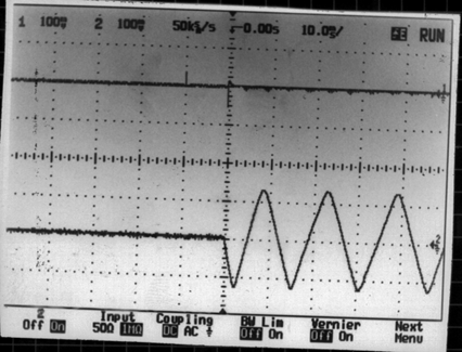
      Fig. 2: SPS phase loop and synchro loop discri at injection. Synchro loop off. Wrong frequency. [12].

       

      

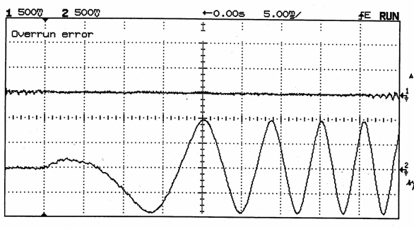
      Fig. 3: SPS phase loop and synchro loop discri at injection. Synchro loop off. Correct frequency but wrong phase. [12].

       

      • In addition the stable phase error can be deduced from an acceleration (increasing beat frequency) or deceleration (decreasing beat frequency).

   5. Coarse adjustment of the Stable Phase to get a constant beat frequency. The beam is neither accelerated nor decelerated.

   6. Then adjust the injection phase to cancel the transient in the Phase Loop phase discri output ΔФ_phase.

   7. Measure the beat frequency, that is the frequency error at injection

    

5. Measure residual energy error and correct

   1. Measure the residual momentum mismatch by observing the phase pick-up signal (sinusoidal oscillation with amplitude proportional to the momentum mismatch)

   2. Re-adjust Bdl_SPS, Bdl_LHC1, Bdl_LHC2, f_{RF SPSLHC}

Step A.2.7: Beam capture and Synchro Loop Commissioning [Interleaved injection] (see Fig 1) [2x8 hours]  [One beam at a time]

• Requires a beam lifetime of about 100 ms (that is about 1000 turns).

1. Commission Synchro Loop

   1. RF Preparation:

      1. Keep RF ON

      2. Leave the Synchro Loop ON at injection

         • As the stable phase error is small (few degrees) and the frequency error is small compared to the loop response (a bit slower than the synchrotron frequency = 60 Hz), the loop should lock: beam is captured.

      3. Keep Phase Loop ON

      4. Keep Radial Loop OFF

   2. Fine tune the injection phase and the stable phase:

      • The injection phase is changed to minimize the phase oscillations at injection (which are in any case damped by the phase loop). As we are on the phase loop, the beam imposes the frequency and might accelerate or decelerate the beam. the stable phase is adjusted to avoid this.

   3. A small frequency error at injection can be deduced from the slope of the Synchro Loop phase discri ΔФ_sync.

    

2. Adjust Synchro Loop dynamics [8 hours]

   1. With both loops ON (Phase Loop and Synchro Loop), measure the synchro loop step response

   2. Adjust the synchro loop gain and phase advance to fine tune the response

   3. Optional at this stage: As this depends on the RF voltage via synchrotron frequency, it should be done at different voltages. This fine tuning at different RF voltages should be done before Phase A.8 (snapback and ramp).

    

3. Optional at this stage: Check phasing of cavity sum [8 hours]

   Note: should be done before before Phase A.8 (snapback and ramp) AND before increasing intensity.

    

   1. Now try to capture the beam with one cavity at a time

   2. Observe synchro loop phase discri output ΔФ_sync after transient

   3. If non-zero, fine-tune the delay in Cavity Sum for that cavity

    

4. Repeat for second ring

    

5. Fine tune capture [2x4 hours]

   1. Voltage matching SPS-LHC:

      1. Observe 400 MHz component of bunch intensity using Bunch Phase module (or APW peak).

      2. Minimize quadrupole oscillations

   2. Measure the bunch profile at injection (using a scope in SR4 or OASIS)

   3. Optional at this stage: Measure the lifetime (using a scope in SR4 or OASIS). Should be done before Phase A.8 (snapback and ramp).

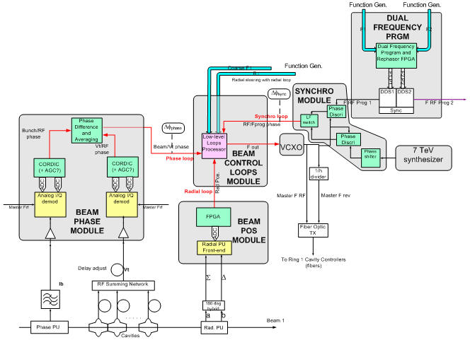
Fig. 1: Low level RF Beam Control Loops [12].

Notes on figure 1:

• Injection frequency, injection phase and stable phase will be adjusted by observing two signals:  ΔФ_phase  and ΔФ_sync .

• A function sets the RF frequency on the injection plateau and through the ramp, via the Dual Frequency Program

• The 7 TeV synthesizer replaces the frequency program during physics

• The VXCO generates the RF sent to the Cavity Controllers