|
Step |
Activity |
Who |
Priority |
|
A.10.1 |
Get Beams into Collision in the X,Y plane |
OP |
1 |
|
.01 |
At the end of the ramp or squeeze (depending on the phase) beams should be separated (~14σ). | ||
|
.02 |
Separator bumps at nominal 0 at all IPs (get settings from best knowledge; beams should be already fairly close). |
|
|
|
.03 |
Measure beam displacement at the IP using BPMs. |
|
|
|
.04 |
Adjust beam separation such that the beam 1 and beam 2 difference left/right of the IP is the same. Do this for one IP at the time. [Note 1] |
|
|
| .05 | Monitor lifetime for all the bunches/empty buckets/abort gap; monitor beam losses. If OK continue, else separate beams. | ||
|
.06 |
"Watch" background. |
|
|
|
.07 |
Change mode from ADJUST to STABLE BEAMS (if lifetime and background under control). | ||
|
.08 |
Start counting delivered luminosity; logging into database (~ Hz). | ||
|
A.10.2 |
Measure and correct longitudinal position |
OP/RF |
2 |
|
.01 |
Shift RF phase to monitor the longitudinal position [Note 2]. | ||
|
A.10.3 |
Monitor lifetime, beam losses and keep background low and stable (no spikes) [Note 3] |
OP |
1 |
|
A.10.4 |
OP/ABP |
2 |
|
|
A.10.5 |
Monitor luminosity during the fill provided by the experiments [Note 5] |
OP |
2 |
|
A.10.6 |
Waist measurement (adjust quads in the triplets) [Note 6] | OP/ABP | If lumi asymmetry in the experiments |
|
A.10.7 |
Measure b* and/or D* and/or IP coupling | OP/ABP | If we have doubts |
|
A.10.8 |
Optimize Luminosity: complementary method; beam-beam transfer function [Note 7] |
OP/ABP |
Backup |
|
A.10.9 |
Absolute luminosity determination: stablish beam size at the IP via extrapolation [Note 8] |
OP/ABP |
3 (Special runs) |
|
A.10.10 |
Absolute luminosity determination: Orthogonal separation scan (Van der Meer) [Note 9] |
OP/ABP |
3 (Special runs) |
Details of activities:
Note 1: Adjust beam separation such that the beam 1 and beam 2 difference left/right of the IP is the same: measure this with special (beam) directional strip line couplers BPMSW at ~ 21 m L/R from the IP in front of Q1.
The expected BPM resolution for small separation and 0 crossing angle in each plane is initially ~ 100 - 200 μm (later and after k modulation ~ 50 μm). However this resolution may be just sufficient to get beams close enough to see some collisions for un-squeezed beams at 7 TeV (for squeezed beams this resolution is not enough) ==> Request for an improved BPM system at the IP (anyway needed for high-beta).
Based on BPM information check that:
|
δr (σ) |
δx,y (σ) |
δx,y (μm) (@ 7 TeV and nominal є) |
|||
| b* = 11m | b* = 2 m | b* = 0.5 m | |||
| To see collisions with resonable luminosity | < 2σ | < 1.4σ | < 133 μm | < 44 μm | < 23 μm |
| To optimize lumi and equalize between experiments | < 0.5σ | < 0.35σ | < 33 μm | < 11 μm | < 6 μm |
Table 1: Beam separation values.
At this point, beams should be colliding.
Alternative method used HERA (by B. Holzer): excite one beam at its tune frequency and observe the spectrum of the other beam. When the beams are close to each other, one can see an increasing amplitude of the excitation frequency in the beam.
Note 2: In principle not too critical in commissioning. Since first collisions will be without crossing angle and with rather large beta* (11 m), even few ns resolution could be sufficient together with information from the experiments. Once in stable physics this will be monitored by the experiments.
How to detect offsets later? : A new electronic card has been developed. Uses the BPMs around the IP and existing infrastructure and allows to measure the relative beam arrival times with sub ns resolution.
Note 3: List of background sources and how they can be minimized [4,5]:
-
Beam gas: good vacuum quality in particular around the experiments.
-
Halo: minimize halo production and maximize cleaning efficiency (well corrected machine, avoid resonances, minimize heating/vibrations) careful transverse feedback, orbit feedback, etc. Optimize lifetime and minimize emittance growth.
-
Physics Collisions: they have side effects that we can minimize: avoid small offsets, e.g. 0.1 σ is negligible for the luminosity (just 0.25% effect), but it may have effects on lifetime/halo since a small fraction of the scattered beam protons can travel to the next IP(s).
HERA procedure on background optimization (by B. Holzer):
-
First of all beams should collide as good as possible: central collisions, max. luminosity is crucial.
-
Optimize the angle of the two beams, again according to the best luminosity, but now also according to the lowest background.
-
Adjust collimators.
-
Optimize the diffusion rate of the beams (crucial). In the case of HERA the ideal tunes were the ones close to the coupling resonance as they suffered even from 12 order resonances under collisions. And close to the diagonal in the tune diagram there was more free place.
-
Tune, chromaticity (small values).
-
Optimize the coupling; if there was a measurable coupling the lifetime in HERA was easily reduced by a factor of 5.
-
The last step was an upstream orbit correction according to the background signals of the experiment.
At HERA the background tuning in general was done as a function of the overall beam loss monitors rate. Although they could have taken the lifetime measurement, in their case it turned out that the loss rate was faster and much more sensitive.
Note 4: The luminosity optimization will be done at least once per fill during the physics runs irrespective of the type of beams: single bunch, multi-bunch, head on collisions, collisions with crossing angle, low intensity, high intensity beams, etc.
During optimization, monitoring of the lifetime of all bunches, the experiments background, the contents of the abort gap and the beam loss monitors shall be mandatory. The scans shall be automatically stopped if any of these signals go above threshold. The abort of a scan and automatic back out to initial values shall be possible.
The application will perform the following steps:
1. Scan the IP in x and y directions using standard separation bumps over ±2σ. The number of steps shall be configurable. The minimum meaningful step size depends on the resolution of the BRAN (Fig. 1) at the given luminosity. For example, 0.2σ gives a 1% change in luminosity which should be detectable by the BRAN at nominal luminosity (see Table 2). A small configurable waiting period shall be used to ensure that the correctors are at appropriate current values.
1. Obtain a series of luminosity measurements from the BRAN detectors participating in the scan. The number of measurements per point shall be configurable. [Cross IP effects could also be monitored.] The average over these measurements shall give a statistical error for each point of scan – to be combined with the error on each measurement coming from the BRAN.
2. The software shall plot the measured luminosity as a function of the separation and fit the results to give the separation bump setting corresponding to the maximum luminosity. Appropriate error analysis shall be performed and displayed.
3. Once the settings giving maximum luminosity are found, the user will have the possibility to set the appropriate value in the control system. These values should then be used as the initial settings in the following run. However, these initial values shall be editable by hand.
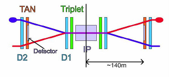
Fig. 1: BRAN Detectors monitor the collision rate by detecting the flux of forward neutral particles generated in the interaction point.
|
Dx(σ) |
Dy(σ) |
L/Lo |
|
0 |
0 |
1 |
|
0.2 |
0 |
0.9901 |
|
0.5 |
0 |
0.9394 |
|
0.5 |
0.5 |
0.8825 |
|
1 |
0 |
0.7788 |
|
1 |
1 |
0.6065 |
Table 2: Change in luminosity as a function of the beam separation [1]. The beam separation is given in units of beam size, σ.
Luminosity optimization at HERA (by B. Holzer): one of the steps in luminosity optimization was "Timing optimization": they had an independent tool to shift the timing of one beam with respect to the other, so to steer the timing of one beam with respect to the other and monitor the luminosity response. This knob was, however, an overall parameter: a timing which was optimal in one collision point was not always the optimum in other collision point. There were always small errors in the length of the storage ring and so it might happen that the length from one IP to next was not exactly the theoretical one.
Note 5: Monitor the delivered luminosity (background subtracted and corrected for any dead-time inefficiency) provided by the experiments.
Note 6: Waist position to optimize and equalize luminosities between experiments: should not be critical in commissioning for unsqueezed optics; beta varies only by 0.8% over a length of ± 1 m from the IP for beta* = 11 m [6,7].
Note 7: This method was successfully used in other machines like DORIS-1[8], ISR[9,10] and HERA[11].
Note 8: This method consists of calculating the emittance via measurement of the beam size at a given point of the ring using a dedicated instrument such a wire scanner, or synchrotron light telescope. Given estimates of the beta function at the location of the device along with the local dispersion, and knowledge of the energy spread, one can extrapolate to the interaction point and use the luminosity formula (Eq. 1) directly. The other key parameters that enter into the equation are the measured beam currents.

Equation 1: luminosity formula that can be applied to the LHC assuming Gaussian distributions for the beam density distribution functions and equal bunch lengths. N1,N2 is the number of particles per bunch for beam 1 and beam 2, respectively; frev is the bunch revolution frequency; Nb is the number of bunches in the beam; σix, σiy is the transverse beam size (i = 1,2).
Note 9: This method uses orthogonal separation scans using the separation scan application [2] described in Note 4. These are commonly referred to as van der Meer scans [13-15] . The absolute luminosity can be obtained by three types of analysis of the data thus obtained:
1. Fit
the measured luminosity as a function of the separation (one direction
at the time), Equation 1 with the contribution of Equation 3 for x and
then y. The result of the fit gives
![]() for
the beam size in the x direction (
for
the beam size in the x direction (![]() for
the y direction).
for
the y direction).
2. Integrate
under the curve of the separation scan distribution, and divide by the
peak relative luminosity to obtain
![]() for the beam size in the x direction (
for the beam size in the x direction (![]() for
the y direction).
for
the y direction).
A scan in each plane is performed. It is generally assumed that the distributions are Gaussian and no crossing angle.
The luminosity calibration scans (methods in Note 8 and Note 9) will be done with much less frequency than the luminosity optimization ones, and they will be performed during dedicated runs with simple beam conditions: few bunches, no crossing angle, low intensity, etc; in order to minimize the source of errors in the measurements. All experiments except the one where the scan is being performed would have separated beams.
From the effective sizes calculated with the methods above (Note 8 and Note 9) the absolute luminosity from machine parameters can be computed. Nevertheless, this implies excellent performance and knowledge of:
• Beam current transformers
• Luminosity monitors
• Machine Optics
• Beam position monitors at the interaction region
• Stability
This procedure also demands care with the measurement precision and error propagation. A dedicated analysis package is needed to take care of this.